A worksheet in Excel is made up of cells. These cells can be referenced by specifying the row value and the column value.
For example, A1 would refer to the first row (specified as 1) and the first column (specified as A). Similarly, B3 would be the third row and second column.
The power of Excel lies in the fact that you can use these cell references in other cells when creating formulas.
Now there are three kinds of cell references that you can use in Excel:
Understanding these different types of cell references will help you work with formulas and save time (especially when copy-pasting formulas).
This Tutorial Covers:
Let me take a simple example to explain the concept of relative cell references in Excel.
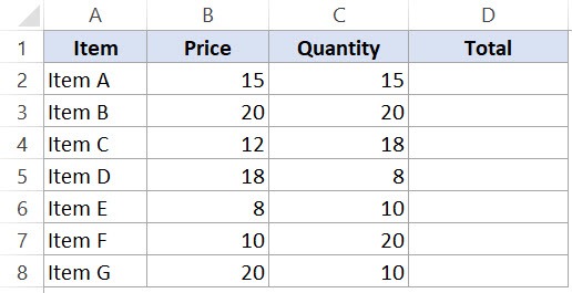
Suppose I have a data set shown below:

To calculate the total for each item, we need to multiply the price of each item with the quantity of that item.
For the first item, the formula in cell D2 would be B2* C2 (as shown below):
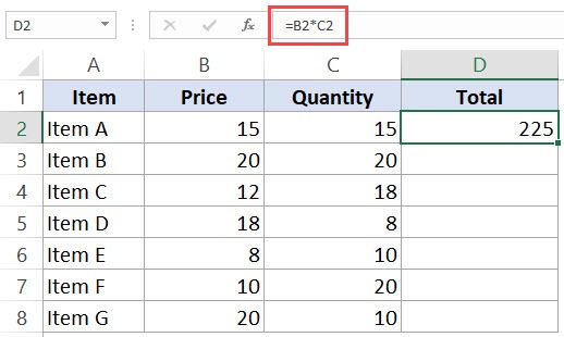
Now, instead of entering the formula for all the cells one by one, you can simply copy cell D2 and paste it into all the other cells (D3:D8). When you do it, you will notice that the cell reference automatically adjusts to refer to the corresponding row. For example, the formula in cell D3 becomes B3*C3 and the formula in D4 becomes B4*C4.
These cell references that adjust itself when the cell is copied are called relative cell references in Excel.
Relative cell references are useful when you have to create a formula for a range of cells and the formula needs to refer to a relative cell reference.
In such cases, you can create the formula for one cell and copy-paste it into all cells.
Unlike relative cell references, absolute cell references don’t change when you copy the formula to other cells.
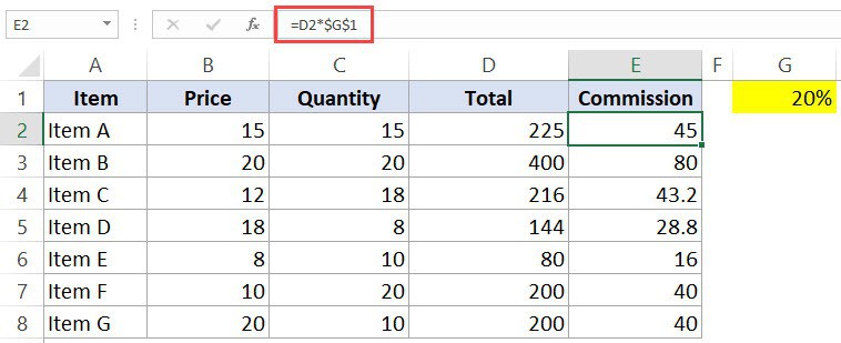
For example, suppose you have the data set as shown below where you have to calculate the commission for each item’s total sales.
The commission is 20% and is listed in cell G1.
 Absolute Cell reference in Excel - Dataset blank" width="760" height="266" />
To get the commission amount for each item sale, use the following formula in cell E2 and copy for all cells:
=D2*$G$1
 Absolute Cell reference in Excel - formula" width="758" height="309" />
Note that there are two dollar signs ($) in the cell reference that has the commission – $G$2.
A dollar symbol, when added in front of the row and column number, makes it absolute (i.e., stops the row and column number from changing when copied to other cells).
For example, in the above case, when I copy the formula from cell E2 to E3, it changes from =D2*$G$1 to =D3*$G$1.
Note that while D2 changes to D3, $G$1 doesn’t change.
Since we have added a dollar symbol in front of ‘G’ and ‘1’ in G1, it wouldn’t let the cell reference change when it’s copied.
Hence this makes the cell reference absolute.
Absolute cell references are useful when you don’t want the cell reference to change as you copy formulas. This could be the case when you have a fixed value that you need to use in the formula (such as tax rate, commission rate, number of months, etc.)
While you can also hard code this value in the formula (i.e., use 20% instead of $G$2), having it in a cell and then using the cell reference allows you to change it at a future date.
For example, if your commission structure changes and you’re now paying out 25% instead of 20%, you can simply change the value in cell G2, and all the formulas would automatically update.
Mixed cell references are a bit more tricky than the absolute and relative cell references.
There can be two types of mixed cell references:
Let’s see how it works using an example.
Below is a data set where you need to calculate the three tiers of commission based on the percentage value in cell E2, F2, and G2.

Now you can use the power of mixed reference to calculate all these commissions with just one formula.
Enter the below formula in cell E4 and copy for all cells.
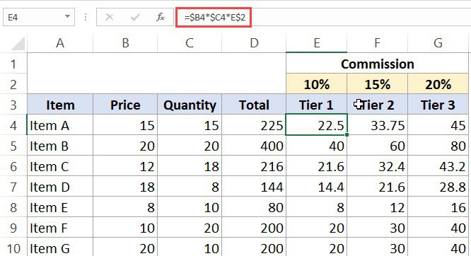
The above formula uses both kinds of mixed cell references (one where the row is locked and one where the column is locked).
Let’s analyze each cell reference and understand how it works:
To change the reference from relative to absolute, you need to add the dollar sign before the column notation and the row number.
For example, A1 is a relative cell reference, and it would become absolute when you make it $A$1.
If you only have a couple of references to change, you may find it easy to change these references manually. So you can go to the formula bar and edit the formula (or select the cell, press F2, and then change it).
However, a faster way to do this is by using the keyboard shortcut – F4.
When you select a cell reference (in the formula bar or in the cell in edit mode) and press F4, it changes the reference.
Suppose you have the reference =A1 in a cell.
Here is what happens when you select the reference and press the F4 key.
You May Also Like the Following Excel Tutorials: